EXECUTIVE OVERVIEW
KNN as a Feature Engine can aid in ensemble learning by quantifying anecdotal knowledge through supervised machine learning.
A good example would be targeting a minority group of customers who are known to have a desirable trait (e.g., similar features/patterns in customer behavior indicative of higher ‘value’ buyers, etc.).
Part one of this two-part series reviews model transformations, metric evaluation, and practices for implementing KNN as a Feature Engine whilst giving users a self-containing script to follow.
THE DETAILS
UPDATE!
Updated code/analysis/video posted to part two of this series.
Please reference this blog for the most up-to-date information!
BACKGROUND:
I wanted to use ‘KNN as a Feature Engine’ as described in O’Reilly’s Practical Statistics for Data Scientists book1 (p.218/247 e2). However, I couldn’t find an example coupling oversampling-data-generation techniques for imbalanced data with feature engineering. Therefore, I decided to publish my own example.
SOLUTION:
I built this model utilizing completely randomized data. Please note, any ‘insights’ found by this model are most likely overfitting the data and will not generalize well2. However, if applied correctly (i.e., utilizing these concepts with real data and intuition) the output can help you build reliable models which will deliver insight and predictions.
TABLE OF CONTENTS:
- THE CODE
- THE MODEL OVERVIEW
- TRAINING THE MODEL
- DEPLOYING THE MODEL (The Results)
- FINAL CONSIDERATIONS
THE CODE
The Model (Coded in R)
##########################
## Establish Environment
##########################
## Packages
  library('pacman')
  pacman::p_load(dplyr, FNN,  performanceEstimation, unbalanced )
## User Defined Parameters
  ## KNN Objectives
    Knn_Output <- 'TEST' ## TEST | MODEL
      # Knn_Output >> Evaluate KNN over Test or model
    KNN_TrainSet_Change <- 'NONE' ## NONE | SCALE | SMOTE | TOMEK | ENN
      # KNN_TrainSet_Change >> Different transformations to be applied to KNN
  ## KNN Parameters
    KNN_K = 3
      # KNN_K >> Run evaluation once (K=1), then run 'TEST-K' script for best K
    SMOTE_PrcOver = 3
    SMOTE_PrcUnder = 1.34
    ENN_K = 3
  ## Dataset Parameters
    df_Size <- 10000 ## Magnitude of 10 (e.g., 10, 100, 1000, etc.)
    df_Imbal <- 0.1 ## Works best <= 0.5
    df_Bias <- 'NONE' ## NONE | BIAS
      ## df_Bias >> None = Completely Random
        ##, Bias = Bias with data (i.e., imbalance class has less variability)
## Data
  set.seed(2023)
  Index <- 1 + (0:(df_Size - 1)) * 1
  df <-
    data.frame(
      IndexID = as.factor(Index)
      ,y=rep(as.factor(c('0','1'))
             ,times=c(ceiling(as.integer(df_Size*(1-df_Imbal)))
                      ,ceiling(as.integer(df_Size*df_Imbal))))
      ,x1=if(df_Bias=='BIAS'){ifelse(Index>(df_Size*(1-df_Imbal))
                                     ,rnorm(df_Size/100)
                                     ,rnorm(df_Size))}else{rnorm(df_Size)}
      ,x2=if(df_Bias=='BIAS'){ifelse(Index>(df_Size*(1-df_Imbal))
                                     ,rnorm(df_Size/100)
                                     ,rnorm(df_Size))}else{rnorm(df_Size)}
    )
##########################
## KNN PREP: Split, Scale, SMOTE, TOMEK, ENN
##########################
##SPLIT
  sample_size = floor(0.8*nrow(df))
  split = sample(seq_len(nrow(df)),size = sample_size)
    train_cl = df[split,]
    test_cl = df[-split,]
## SCALE
  train_scale <- scale ( train_cl[,3:4] )
  test_scale <- scale ( test_cl[,3:4] )
## SMOTE
  train_scale_smote <-
    performanceEstimation::smote(
      y ~ x1 + x2
      , data= mutate( as.data.frame( train_scale)
      , y = train_cl[,2])
      , perc.over = SMOTE_PrcOver, perc.under = SMOTE_PrcUnder )
## TOMEK
  Tomek <- ubTomek( train_scale_smote[,-3], train_scale_smote[,3] )
    train_scale_smote_TOMEK <- cbind(Tomek$Y, Tomek$X)
    colnames( train_scale_smote_TOMEK) <- c("y", "x1" , "x2")
## ENN
  ENN <- ubENN( train_scale_smote[,-3], train_scale_smote[,3] , k = ENN_K )
    train_scale_smote_ENN <- cbind(ENN$Y, ENN$X)
    colnames( train_scale_smote_ENN) <- c("y", "x1" , "x2")
##########################
## KNN (Training)
##########################
## KNN Evaluation Parameters
  KNN_Train <-
    if ( KNN_TrainSet_Change == 'NONE' ) {train_cl[,3:4]} else
      if ( KNN_TrainSet_Change == 'SCALE' ) { train_scale } else
      if ( KNN_TrainSet_Change == 'SMOTE' ) { train_scale_smote[,-3] } else
      if ( KNN_TrainSet_Change =='TOMEK' ) { train_scale_smote_TOMEK[,-1] }else
      if ( KNN_TrainSet_Change == 'ENN' ) { train_scale_smote_ENN[,-1] }
  KNN_TrainClass  <-
    if ( KNN_TrainSet_Change == 'NONE' ) {train_cl[,2]} else
      if ( KNN_TrainSet_Change == 'SCALE' ) { train_cl[,2] } else
      if ( KNN_TrainSet_Change == 'SMOTE' ) { train_scale_smote[,3] } else
      if ( KNN_TrainSet_Change =='TOMEK' ) { train_scale_smote_TOMEK[,1] } else
      if ( KNN_TrainSet_Change == 'ENN' ) { train_scale_smote_ENN[,1] }
  KNN_Test_Test <- if ( KNN_TrainSet_Change %in% c ( 'NONE' ) )
    { test_cl[,3:4]} else { test_scale }
  KNN_Test_Train <- if ( KNN_TrainSet_Change %in% c ( 'NONE' ) )
    { train_cl[,3:4] } else { train_scale }
## KNN (Training)
  KNN_classifier_test <-
    knn( train = KNN_Train , test = KNN_Test_Test , cl = KNN_TrainClass
         , prob = TRUE, k = KNN_K )
## Confusion Matrix & Metrics
  if ( Knn_Output == 'TEST' )
  { cm <- table(test_cl[,2], KNN_classifier_test)
    print ( cm )
      Accuracy <- round( (cm[1,1]+cm[2,2]) / sum(cm[]), digits = 4) * 100
      Precision <- round( cm[2,2] / sum(cm[,2]), digits = 4)* 100
      Specificity <- round( cm[1,1] / sum(cm[1,]), digits = 4)* 100
      Recall <- round( cm[2,2] / sum(cm[2,]), digits = 4)* 100
      FScore <- round(2*((Precision*Recall)/(Precision+Recall)),digits=2)
    print(paste('Accuracy=',Accuracy,'% | Precision=',Precision
                ,'% | Specificity=',Specificity,'% | Recall='
                ,Recall,'% | FScore=',FScore,'%') )
  }
##########################
## KNN as a Feature Engine || PSEUDO-LABELING/SELF-TRAINING
##########################
  if ( Knn_Output == 'MODEL') {
    ## KNN - TRAIN DATASET
      KNN_classifier_train <-
        knn(train=KNN_Train,test=KNN_Test_Train,cl=KNN_TrainClass
            ,prob=TRUE,k=KNN_K )
    ## Feature Engineering
        test_cl$Class <- KNN_classifier_test
        test_cl$ClassScore <- attr(KNN_classifier_test, "prob" )
        train_cl$Class <- KNN_classifier_train
        train_cl$ClassScore <- attr(KNN_classifier_train, "prob")
      ## Merge with Original
        df_final <- rbind ( train_cl , test_cl )
          df_final <- df_final[c("IndexID", "Class", "ClassScore")]
          df_final <- merge( df , df_final , by = c("IndexID") )
          df_final <- df_final[order(df_final$IndexID),]
  ## Confusion Matrix & Metrics
      cm <- table(df_final[,2], df_final[,5])
      print ( cm )
        Accuracy <- round( (cm[1,1]+cm[2,2]) / sum(cm[]), digits = 4) * 100
        Precision <- round( cm[2,2] / sum(cm[,2]), digits = 4)* 100
        Specificity <- round( cm[1,1] / sum(cm[1,]), digits = 4)* 100
        Recall <- round( cm[2,2] / sum(cm[2,]), digits = 4)* 100
        FScore <- round(2*((Precision*Recall)/(Precision+Recall)),digits=2)
      print(paste('Accuracy=',Accuracy,'% | Precision=',Precision
                ,'% | Specificity=',Specificity,'% | Recall='
                ,Recall,'% | FScore=',FScore,'%') )
  }
Testing K (Coded in R)
## KNN = 3
  KNN_classifier_test <-
    knn(train=KNN_Train,test=KNN_Test_Test,cl=KNN_TrainClass,prob=TRUE,k=3)
  cm <- table(test_cl[,2], KNN_classifier_test)
    Accuracy <- round( (cm[1,1]+cm[2,2]) / sum(cm[]), digits = 4) * 100
    Precision <- round( cm[2,2] / sum(cm[,2]), digits = 4)* 100
    Specificity <- round( cm[1,1] / sum(cm[1,]), digits = 4)* 100
    Recall <- round( cm[2,2] / sum(cm[2,]), digits = 4)* 100
    FScore <- round(2*((Precision*Recall)/(Precision+Recall)),digits=2)
  print(paste('KNN = 03:','Accuracy=',Accuracy,'% | Precision=',Precision
          ,'% | Specificity=',Specificity,'% | Recall=',Recall
          ,'% | FScore=',FScore,'%'))
## KNN = 5
  KNN_classifier_test <-
    knn(train=KNN_Train,test=KNN_Test_Test,cl=KNN_TrainClass,prob=TRUE,k=5)
  cm <- table(test_cl[,2], KNN_classifier_test)
    Accuracy <- round( (cm[1,1]+cm[2,2]) / sum(cm[]), digits = 4) * 100
    Precision <- round( cm[2,2] / sum(cm[,2]), digits = 4)* 100
    Specificity <- round( cm[1,1] / sum(cm[1,]), digits = 4)* 100
    Recall <- round( cm[2,2] / sum(cm[2,]), digits = 4)* 100
    FScore <- round(2*((Precision*Recall)/(Precision+Recall)),digits=2)
  print(paste('KNN = 05:','Accuracy=',Accuracy,'% | Precision=',Precision
          ,'% | Specificity=',Specificity,'% | Recall=',Recall
          ,'% | FScore=',FScore,'%'))
## KNN = 7
  KNN_classifier_test <-
    knn(train=KNN_Train,test=KNN_Test_Test,cl=KNN_TrainClass,prob=TRUE,k=7)
  cm <- table(test_cl[,2], KNN_classifier_test)
    Accuracy <- round( (cm[1,1]+cm[2,2]) / sum(cm[]), digits = 4) * 100
    Precision <- round( cm[2,2] / sum(cm[,2]), digits = 4)* 100
    Specificity <- round( cm[1,1] / sum(cm[1,]), digits = 4)* 100
    Recall <- round( cm[2,2] / sum(cm[2,]), digits = 4)* 100
    FScore <- round(2*((Precision*Recall)/(Precision+Recall)),digits=2)
  print(paste('KNN = 07:','Accuracy=',Accuracy,'% | Precision=',Precision
          ,'% | Specificity=',Specificity,'% | Recall=',Recall
          ,'% | FScore=',FScore,'%'))
## KNN = 15
  KNN_classifier_test <-
    knn(train=KNN_Train,test=KNN_Test_Test,cl=KNN_TrainClass,prob=TRUE,k=15)
  cm <- table(test_cl[,2], KNN_classifier_test)
    Accuracy <- round( (cm[1,1]+cm[2,2]) / sum(cm[]), digits = 4) * 100
    Precision <- round( cm[2,2] / sum(cm[,2]), digits = 4)* 100
    Specificity <- round( cm[1,1] / sum(cm[1,]), digits = 4)* 100
    Recall <- round( cm[2,2] / sum(cm[2,]), digits = 4)* 100
    FScore <- round(2*((Precision*Recall)/(Precision+Recall)),digits=2)
  print(paste('KNN = 015:','Accuracy=',Accuracy,'% | Precision=',Precision
          ,'% | Specificity=',Specificity,'% | Recall=',Recall
          ,'% | FScore=',FScore,'%'))
## KNN = 19
  KNN_classifier_test <-
    knn(train=KNN_Train,test=KNN_Test_Test,cl=KNN_TrainClass,prob=TRUE,k=19)
  cm <- table(test_cl[,2], KNN_classifier_test)
    Accuracy <- round( (cm[1,1]+cm[2,2]) / sum(cm[]), digits = 4) * 100
    Precision <- round( cm[2,2] / sum(cm[,2]), digits = 4)* 100
    Specificity <- round( cm[1,1] / sum(cm[1,]), digits = 4)* 100
    Recall <- round( cm[2,2] / sum(cm[2,]), digits = 4)* 100
    FScore <- round(2*((Precision*Recall)/(Precision+Recall)),digits=2)
  print(paste('KNN = 19:','Accuracy=',Accuracy,'% | Precision=',Precision
          ,'% | Specificity=',Specificity,'% | Recall=',Recall
          ,'% | FScore=',FScore,'%'))
THE MODEL OVERVIEW
Before we dive in, I wanted to recognize GeeksForGeeks for their easy-to-understand KNN layout3, Statology for their imbalanced dataset example4, and OpenAI for their ChatGPT bot whom unstuck me5 , accelerated my learnings, and whom I will be referencing quite a few times!
Establishing The Environment
There are three subsections: Packages, User Defined Parameters, and the Data itself.
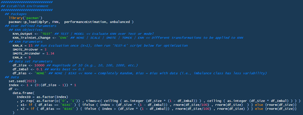
Packages:
- I utilized the packman package which will load subsequent packages and their dependents through the p_load function; this makes the code easier to read/share6.
- I used a depreciated package ‘unbalanced’ for its ease of use, understanding, and robustness. ChatGPT gave the best response for loading these packages. Simply, (1) download the archived package and (2) load the “.tar.gz” file directly into R studio. Please note, depreciated packages have their downsides (e.g., unsupported, compatibility issues, etc.) – so productionizing these packages will need to be evaluated with serious consideration.
User Defined Parameters
User Defined Parameters can be split into three subsections: KNN Objectives, KNN Parameters, and the Dataset Parameters.
- KNN Objectives:
- KNN_Output: This is indicative of user intent. If the user wants to evaluate and train their model over the test set, then choose ‘TEST’. If the user is ready to deploy their model and add KNN as a feature engine to their base dataset, then choose ‘MODEL’.
- KNN_TrainSet_Change: This allows users to update the training set for their desired evaluation.
- None: no change to train set
- Scale: scales train set
- SMOTE: applies SMOTE to scaled train set
- TOMEK/ENN: applies TOMEK/ENN to the SMOTE-SCALE-Training set
- KNN Parameters:
- KNN_K: Run the evaluation once with KNN = 1 to ‘load’ your model into memory. Then, run the ‘Test-K’ script to find the best K value for your model. Insert the best K parameter here.
- SMOTE_PrcOver: This is the third argument for smote{ PerformanceEstimation}. This is the percentage added to the original minority for over-sampling. More information from the technical document.
- SMOTE_PrcUnder: This is the fifth argument smote{ PerformanceEstimation}. This is an under-sampling method that adjusts the majority group based on the ‘PrcOver’ number. I will speak on this more in the ‘KNN PREP’ section, but for now, here is the technical document.
- ENN_K: This is the third parameter for ubENN{unbalanced}. This dictates the number of neighbors used in the evaluation. More information can be found in the unbalanced technical document.
- Dataset Parameters
- df_Size: Updates the size of randomized model to this value.
- df_Imbal: Updates imbalance for model (e.g., you are looking for a 10% vs. 50% rare-case occurrence).
- df_Bias: This adds bias in the model by reducing variability in the rare-class values. Currently, I would not recommend using this feature (protype feature).
Data
Based on the output above, a random dataset will be generated. IndexID is the primary key, Y is the dependent variable, and X1/X2 are the independent variables. Here is a simple breakdown about variables from nces.ed.gov.
KNN Preparation

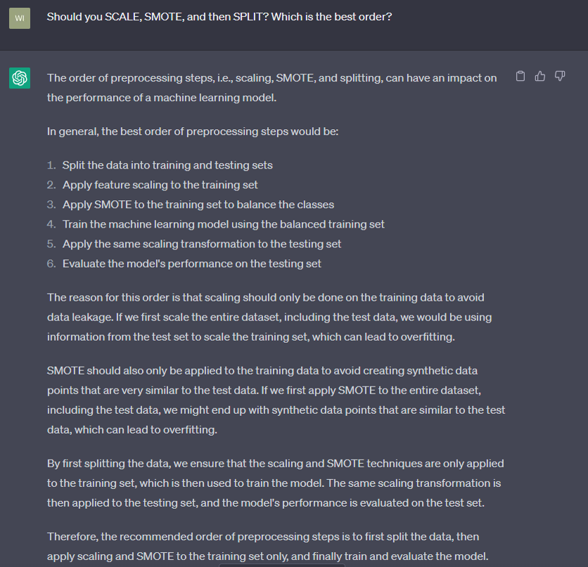
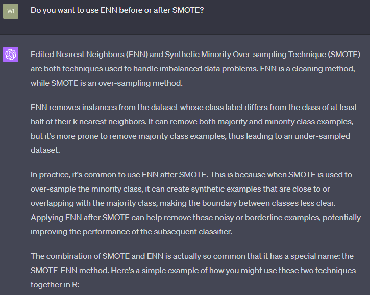
This section performs the standard transformations when dealing with imbalanced datasets. SPLIT partitions the data into an 80/20 split between training and testing. SCALE normalizes the SPLIT data, which means KNN evaluations are not biased based on the scale of the original data, but rather evaluated based on their distribution from the mean (Bruce & Bruce, P.215)1. SMOTE is an oversampling technique where the minority data are synthetically produced to balance the data7. This typically happens over the training dataset. TOMEK & ENN are undersampling techniques that, when combined with SMOTE, clean the areas around class boundaries8; Towards Data Science first introduced me to this hybrid approach9. Frankly, ChatGPT did an excellent job in summarizing the sequence of events, attached are two screen shots for your review:
A quick note is that there will be variability in the output depending on the parameters set for each transformation. These parameters can be fine-tuned by the data analyst or optimized through automated hyperparameter tuning techniques. For instance, the SPLIT ratio can be adjusted to partition the data differently, SMOTE can be modified to alter the oversampling representation (e.g., 10%, 25%, or 50% minority representation), and ENN can be adjusted to consider different numbers of nearest neighbors (K). Each adjustment, or ‘lever,’ can impact the output and effectiveness of the model. Although I won’t delve into hyperparameter tuning in this article, I hope to do so in future post. Meanwhile, here is a helpful blog post on the topic from cran.r-project.org. (This paragraph was edited with ChatGPT for coherence)
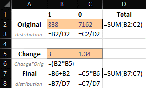
Here’s an additional note regarding the ‘smote’ function within the ‘PerformanceEstimation’ package —when setting parameters, I found it useful to construct a matrix. Take, for example, a situation where the original training data has a 10% minority-class imbalance. In this case, you can calculate the final output by multiplying this 10% by the SMOTE_PrcOver parameter and then adding back the original value. For the SMOTE_PrcUnder parameter, you would take the change value derived from the SMOTE_PrcOver operation (that is, the original imbalance proportion multiplied by the change) and multiply this by the SMOTE_PrcUnder parameter to obtain the final value. (This paragraph was edited with ChatGPT for coherence)
This explanation may seem complex, so I’ve included a visual below to aid in understanding the process:
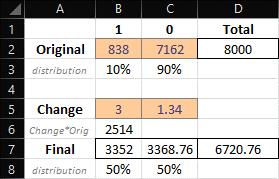
Later in this post, we will see how each parameter change (e.g., SMOTE distribution) will impact the efficacy of the data model.
KNN (Model Training)

There are three subsections to review: KNN Evaluation Parameters, KNN (Training), Confusion Matrix & Metrics
- KNN Evaluation Parameters: This considers the users intended evaluation in the ‘User Defined Parameters’ (above) and produces KNN based on those requirements (e.g., evaluate a SMOTE model with 50% minority distribution over the TEST set).
- KNN (Training): This is where a user trains their model. Ingested parameters are evaluated against the ‘test’ dataset. A few considerations/learnings:
- ‘Prob = TRUE’ ensures you can pull the ‘prob’ attribute utilized for scoring the model.
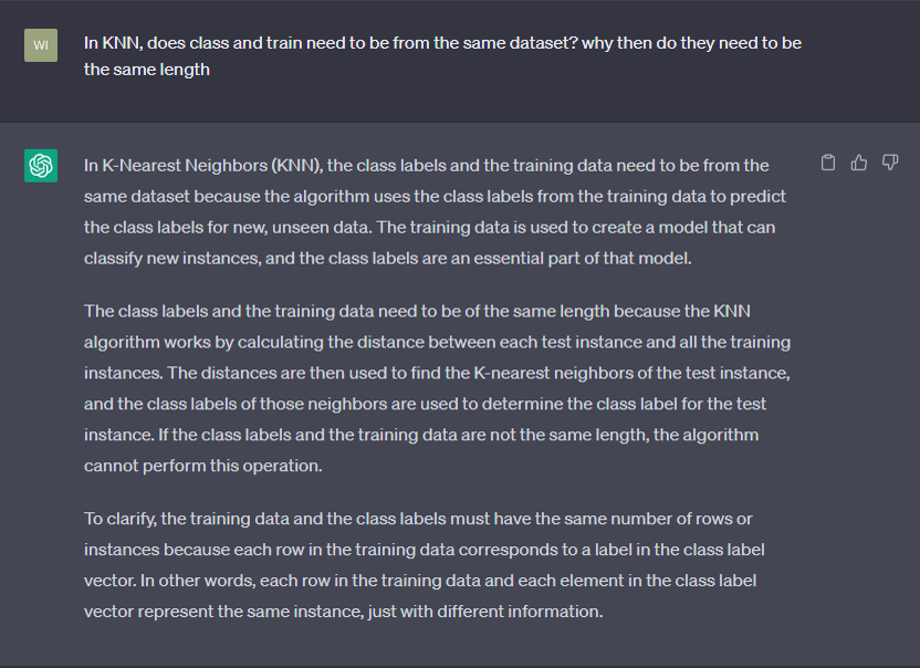
- A huge revelation which was revealed to me was that the train & class (TrainClass) need to be of the same relevance. An example could be that train and class are pulled from the same dataset/data-frame. Train are the independent variables and class are the dependent variables. Even if the train dataset is altered, the respective class dataset still needs to be tied to it. For example, SCALE only factors numeric values (i.e., the factor dependent variable is not included); however, KNN will take the scaled independent values from SCALE and regress them against the non-scaled values from the original split data. All this to say, train and class are tied together and predict the Test & TestClass variables (TestClass hardcoded) which are also tied together. Here is an excerpt from ChatGPT that greatly helped me understand this concept:
- Confusion Matrix & Metrics
- The metrics we’re about to discuss are crucial for evaluating this model. To ensure a valid interpretation, they should be reviewed in their entirety, since a one-sided examination can distort the perception of model ‘accuracy’, leading to a false sense of confidence. For instance, a model may appear to be approximately 90% ‘accurate’, yet only yield a true-prediction rate of around 5% when applied. Several articles delve into the intricacies of various metrics in a confusion matrix (example article: TowardsDataScience). However, the metrics we’ll be focusing on today include:
- Recall: This measures the model’s ability to correctly identify positive instances. In other words, it is the proportion of actual positive cases that the model correctly predicted as positive (Definition adjusted with ChatGPT)
- Precision: This is the proportion of positive predictions that were indeed correct.
- F-Score: This harmonizes the positive and negative metrics into a single score, providing a balanced measure of the model’s performance. Generally, a higher F-Score is preferable.
- The metrics we’re about to discuss are crucial for evaluating this model. To ensure a valid interpretation, they should be reviewed in their entirety, since a one-sided examination can distort the perception of model ‘accuracy’, leading to a false sense of confidence. For instance, a model may appear to be approximately 90% ‘accurate’, yet only yield a true-prediction rate of around 5% when applied. Several articles delve into the intricacies of various metrics in a confusion matrix (example article: TowardsDataScience). However, the metrics we’ll be focusing on today include:
KNN as a Feature Engine
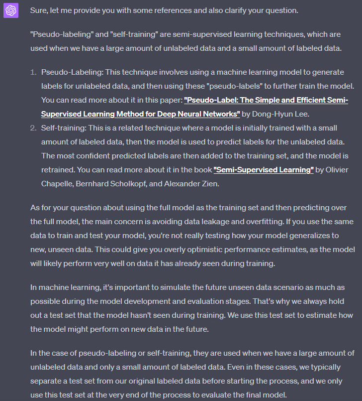
This section diverges from the approach found in O’Reilly’s Practical Statistics for Data Scientists. In the book, so it seemed, the authors test and train over the full dataset before returning the data directly back to the original dataset (Bruce & Bruce, p.218). When presented with the idea, ChatGPT recommended training the model over training data only – a concept common with “Feature Engine” (also called Pseudo-labeling or Self-Training). This approach avoids data leakage introduced when a model is trained over itself. See a ChatGPT excerpt below detailing Pseudo-labeling and data leakage:
Therefore, to effectively mitigate against data-leakage, we evaluate the training set and testing set separately (both over the training model) and merge the two to obtain the predictions for the full model. Because the data was randomly split, we need a way to amalgamate this new dataset with the original dataset. This is why the IndexID column was generated, as it acts as a primary/surrogate key. Finally, when merged back, a confusion matrix is generated with performance metrics to evaluate the final end-state.
This leads to the article’s apex— we can use the output of KNN for ensemble learning. This will be covered further in our second post. For now, we have covered the model in its entirety and will be demonstrating training and evaluating the model.
TRAINING THE MODEL
TRAINING THE MODEL: Randomized Control
As stated earlier, the code is strategically fitting random data. However, it is still of some value to quantify that fit. We will do that by establishing a control and evaluating against that control. In this instance, we will be randomly assigning predicted Y values to the dataset, and this will be used as our randomized control.

We can see that the model accurately predicts the minority value (i.e., y=1) 49.4% of the time (recall), however, precision is very low (i.e., only 10% of total y=1 predictions were correct). It’s good to have a base to reference if we are better than random chance. Now then, let’s move onto the training and deployment of our model.
TRAINING THE MODEL: Constant Parameters
Let’s establish the base dataset parameters (note, these were also used in the randomized control).
- Dataset: Size = 10,000 | Imbalance = 10% | Bias = NONE
- KNN_K = 3
KNN_K = 3 will be constant during the training phase to highlight differences in each evaluation type. However, we will also show the results of testing K to find the best model for our deployment.
TRAINING THE MODEL (Training Set Change = NONE)
- Parameters: Knn_Output = TEST | KNN_TrainSet_Change = NONE
- Model Output: Accuracy = 89.95% | Precision = 14.55% | Specificity = 97.44% | Recall = 4.94% | FScore = 7.38%
- Testing K:
- KNN = 03: Accuracy = 89.95% | Precision = 14.55% | Specificity = 97.44% | Recall = 4.94% | FScore = 7.38%
- KNN = 05: Accuracy = 91.2% | Precision = 6.25% | Specificity = 99.18% | Recall = 0.62% | FScore = 1.13%
- KNN = 07: Accuracy = 91.65% | Precision = 14.29% | Specificity = 99.67% | Recall = 0.62% | FScore = 1.19%
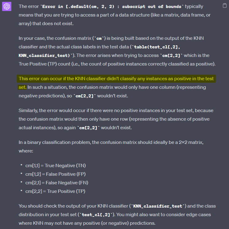
- OTHER KNNS HAD ERROR: “Error in `[.default`(cm, 2, 2) : subscript out of bounds”
- Notes:
- BEST K for KNN_TrainSet_Change = NONE is 3
- Note how accuracy is high at nearly 90%; however, recall is less than 5%. We have talked about this before and will review it again later. Just know, this is where that example comes from 😉
- There is an error message as the model cannot predict any positive values when K is greater than 7 (in our example). Here is ChatGPT explaining this phenomenon:
TRAINING THE MODEL (Training Set Change = SCALE)
- Parameters: Knn_Output = TEST | KNN_TrainSet_Change = SCALE
- Model Output: Accuracy = 89.68% | Precision = 10.53% | Specificity = 97.23% | Recall = 3.7% | FScore = 5.48%
- Testing K:
- KNN = 03: Accuracy = 89.68% | Precision = 10.53% | Specificity = 97.23% | Recall = 3.7% | FScore = 5.48%
- KNN = 05: Accuracy = 91.5% | Precision = 25% | Specificity = 99.35% | Recall = 2.47% | FScore = 4.5%
- KNN = 07: Accuracy = 91.65% | Precision = 22.22% | Specificity = 99.62% | Recall = 1.23% | FScore = 2.33%
- OTHER KNNS HAD ERROR: “Error in `[.default`(cm, 2, 2) : subscript out of bounds”
- Notes:
- Best K for KNN_TrainSet_Change = SCALE is 3
- Note how nearly all metrics are worse compared with the base. I’m going to assume this is due to the nature of the data and its scale. However, scaling (normalizing) the data is still typically the best practice.
- Same K error as before— see notes above.
TRAINING THE MODEL (Training Set Change = SMOTE)
- Parameters: Knn_Output = TEST | KNN_TrainSet_Change = SMOTE | SMOTE_PrcOver = 3 | SMOTE_PrcUnder = 1.34
- Model Output: Accuracy = 57.4% | Precision = 7.82% | Specificity = 58.98% | Recall = 39.51% | FScore = 13.06%
- Testing K:
- SMOTE Distribution = 25% (Over = 3, Under = 4)
- KNN = 03: Accuracy = 75.6% | Precision = 8.84% | Specificity = 80.36% | Recall = 21.6% | FScore = 12.55%
- KNN = 05: Accuracy = 77.5% | Precision = 9.32% | Specificity = 82.54% | Recall = 20.37% | FScore = 12.79%
- KNN = 07: Accuracy = 78.65% | Precision = 9.48% | Specificity = 83.9% | Recall = 19.14% | FScore = 12.68%
- KNN = 15: Accuracy = 83.85% | Precision = 8.72% | Specificity = 90.32% | Recall = 10.49% | FScore = 9.52%
- KNN = 19: Accuracy = 85.2% | Precision = 11.05% | Specificity = 91.68% | Recall = 11.73% | FScore = 11.38%
- SMOTE Distribution = 33% (Over = 3, Under = 2.7)
- KNN = 03: Accuracy = 71.2% | Precision = 8.6% | Specificity = 75.14% | Recall = 26.54% | FScore = 12.99%
- KNN = 05: Accuracy = 71.2% | Precision = 8.43% | Specificity = 75.19% | Recall = 25.93% | FScore = 12.72%
- KNN = 07: Accuracy = 72.6% | Precision = 9.62% | Specificity = 76.5% | Recall = 28.4% | FScore = 14.37%
- KNN = 15: Accuracy = 76.5% | Precision = 9.04% | Specificity = 81.39% | Recall = 20.99% | FScore = 12.64%
- KNN = 19: Accuracy = 77.9% | Precision = 8.08% | Specificity = 83.3% | Recall = 16.67% | FScore = 10.88%
- SMOTE Distribution = 50% (Over = 3, Under = 1.34)
- KNN = 03: Accuracy = 57.4% | Precision = 7.82% | Specificity = 85.98% | Recall = 39.51% | FScore = 13.06%
- KNN = 05: Accuracy = 56.75% | Precision = 8% | Specificity = 58.11% | Recall = 41.36% | FScore = 13.41%
- KNN = 07: Accuracy = 55.95% | Precision = 8.25% | Specificity = 57.02% | Recall = 43.83% | FScore = 13.89%
- KNN = 15: Accuracy = 57.15% | Precision = 8.68% | Specificity = 58.22% | Recall = 45.06% | FScore = 14.56%
- KNN = 19: Accuracy = 56.3% | Precision = 8.51% | Specificity = 57.29% | Recall = 45.06% | FScore = 14.32%
- SMOTE Distribution = 25% (Over = 3, Under = 4)
- Notes:
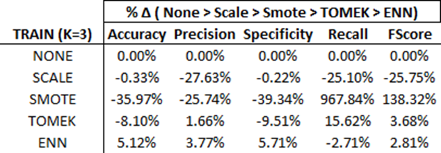
- When K = 3, the F-Score and Recall significantly improved, to the tune of ~138% and ~970% respectively! Note how accuracy took a large hit; this is okay as we would rather have a more well-rounded model (e.g., 99% accuracy with 0% recall is of no use).
- Because SMOTE has parameters, we tested K with a few SMOTE distributions to see which yielded the best F-Score. The SMOTE distribution of 50% with KNN=15 is going to yield the best SMOTE model.
TRAINING THE MODEL (Training Set Change = TOMEK)
- Parameters: Knn_Output = TEST | KNN_TrainSet_Change = TOMEK
- Model Output: Accuracy = 52.75% | Precision = 7.95% | Specificity = 53.37% | Recall = 45.68% | FScore = 13.54%
- Testing K:
- KNN = 03: Accuracy = 52.75% | Precision = 7.95% | Specificity = 53.37% | Recall = 45.68% | FScore = 13.54%
- KNN = 05: Accuracy = 50.5% | Precision = 7.84% | Specificity = 50.76% | Recall = 47.53% | FScore = 13.46%
- KNN = 07: Accuracy = 50% | Precision = 8.02% | Specificity = 50.05% | Recall = 49.38% | FScore = 13.8%
- KNN = 15: Accuracy = 49.15% | Precision = 8.45% | Specificity = 48.75% | Recall = 53.7% | FScore = 14.6%
- KNN = 19: Accuracy = 46.85% | Precision = 8.33% | Specificity = 46.08% | Recall = 55.56% | FScore = 14.49%
- Notes:
- TOMEK improved the F-Score and Recall by 3.68% and 15.62% respectively.
- The best K for TOMEK is k=15
TRAINING THE MODEL (Training Set Change = ENN)
- Parameters: Knn_Output = TEST | KNN_TrainSet_Change = ENN | ENN_K = 9
- Model Output: Accuracy = 55.45% | Precision = 8.25% | Specificity = 56.42% | Recall = 44.44% | FScore = 13.92%
- Testing K:
- ENN_K = 3
- KNN = 03: Accuracy = 55.45% | Precision = 8.25% | Specificity = 56.42% | Recall = 44.44% | FScore = 13.92%
- KNN = 05: Accuracy = 53.85% | Precision = 8.05% | Specificity = 54.62% | Recall = 45.06% | FScore = 13.66%
- KNN = 07: Accuracy = 53.55% | Precision = 8.09% | Specificity = 54.24% | Recall = 45.68% | FScore = 13.75%
- KNN = 15: Accuracy = 52.75% | Precision = 8.48% | Specificity = 53.05% | Recall = 49.38% | FScore = 14.47%
- KNN = 19: Accuracy = 51.3% | Precision = 8.4% | Specificity = 51.36% | Recall = 50.62% | FScore = 14.41%
- ENN_K = 7
- KNN = 03: Accuracy = 57.1% | Precision = 7.97% | Specificity = 58.54% | Recall = 40.74% | FScore = 13.33%
- KNN = 05: Accuracy = 56.45% | Precision = 8.05% | Specificity = 57.73% | Recall = 41.98% | FScore = 13.51%
- KNN = 07: Accuracy = 55.7% | Precision = 8.2% | Specificity = 56.75% | Recall = 43.83% | FScore = 13.85%
- KNN = 15: Accuracy = 56.4% | Precision = 8.72% | Specificity = 57.29% | Recall = 46.3% | FScore = 14.68%
- KNN = 19: Accuracy = 55.55% | Precision = 8.55% | Specificity = 56.37% | Recall = 46.3% | FScore = 14.43%
- ENN_K = 9
- KNN = 03: Accuracy = 57.35% | Precision = 7.92% | Specificity = 58.87% | Recall = 40.12% | FScore = 13.23%
- KNN = 05: Accuracy = 56.6% | Precision = 8.08% | Specificity = 57.89% | Recall = 41.98% | FScore = 13.55%
- KNN = 07: Accuracy = 55.85% | Precision = 8.23% | Specificity = 56.91% | Recall = 43.83% | FScore = 13.86%
- KNN = 15: Accuracy = 56.85% | Precision = 8.81% | Specificity = 57.78% | Recall = 46.3% | FScore = 14.8%
- KNN = 19: Accuracy = 56.05% | Precision = 8.55% | Specificity = 56.96% | Recall = 45.68% | FScore = 14.4%
- ENN_K = 3
- Notes:
- Note how the ENN with KNN_K=3 improved the F-Score again by 2.81% versus TOMEK.
- • As with SMOTE, ENN has parameters that can be tuned. We tested K with multiple ENN_K parameters and found the best combination was ENN_K = 9 and KNN_K = 15. Not only is this the best ENN model, but it’s the best model overall.
TRAINING THE MODEL: Training Overview
Below is the overview of each model over the training data:
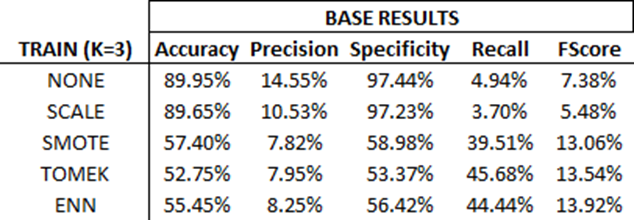
As mentioned prior, notice how no changes to the training set yields the highest ‘accuracy’. This is because the model will be good at predicting true negatives. However, when trying to predict true positives (Recall), one will apply this model and see they are only predicting true positives 4.94% of the time! This is why reviewing other metrics in tandem with accuracy is important.
Also notice how the F-score is increasing with each transformation. This isn’t always the case, but in this example – it’s good to see that each incremental transformation adds value to the model’s predictive strength.
Overall, for this dataset, the ENN transformation yields the highest F-Score. We will deploy this model and measure the results against our randomized control.
Also note, below are the percentage changes from model to model. I have referenced them in prior sections. Here they are for your review:
DEPLOYING THE MODEL (The Results)
As stated earlier, the ENN model with parameters ENN_K = 9 and KNN_K = 15 yielded the highest F-score. We will use this model to make predictions over the whole dataset and generate our factor engine for ensemble learning (i.e., part two of this series).
For now, let’s review the output of the ENN (KNN) model and compare that against our randomized control.
ENN vs Random Control:

As you can see, we added a lot of predictive value through the training transformation. From synthetically creating new minority datapoints (SMOTE) to under-sampling for distinguishing K boundaries (ENN) – this model substantially outperforms the randomized control on every metric.
FINAL CONSIDERATIONS
A few edifications would make this model stronger: hyperparameter tuning and distinguishing a better Train/Test/Validation set.
For hyperparameter tuning, I would seek to automate the optimization of selecting the right parameters. Examples would be optimizing K in KNN and the SMOTE distribution.
For the Train/Test/Validation sets, it’s good to have a Train and Test set as we did in this model, and another hold out to perform validation. There doesn’t seem to be a “hard-fast” rule about sizes, but representation is important. For example, a 98-1-1 distribution on a very large data set might be okay, while a 60-20-20 distribution might be better for smaller data. Here is a helpful article from v7labs: Train Test Validation Split: How To & Best Practices [2023].
REFERENCES
- “Practical Statistics for Data Scientists”, Peter Bruce & Andrew Bruce, (Amazon Affiliate Link) https://amzn.to/3OIQe5z
- “Generalization and Overfitting”, Western Washington University, https://wp.wwu.edu/machinelearning/2017/01/22/generalization-and-overfitting/
- “K-NN Classifier in R Programming”, GeeksForGeeks, https://www.geeksforgeeks.org/k-nn-classifier-in-r-programming/
- “How to Use SMOTE for Imbalanced Data in R (With Example)”, Statology, https://www.statology.org/smote-in-r/
- “KNN as Feature Engine – Tie back to base dataset after SMOTE”, StackOverflow, https://stackoverflow.com/questions/76214393/knn-as-feature-engine-tie-back-to-base-dataset-after-smote
- “An efficient way to install and load R packages”, Stats and R, https://statsandr.com/blog/an-efficient-way-to-install-and-load-r-packages/
- “SMOTE for Imbalanced Classification with Python”, Machine Learning Mastery, https://machinelearningmastery.com/smote-oversampling-for-imbalanced-classification/
- “Overcoming Class Imbalance using SMOTE Techniques”, Analytics Vidhya, https://www.analyticsvidhya.com/blog/2020/10/overcoming-class-imbalance-using-smote-techniques/
- “Stop using SMOTE to handle all your Imbalanced Data”, Towards Data Science, https://towardsdatascience.com/stop-using-smote-to-handle-all-your-imbalanced-data-34403399d3be

