Table of Contents
- Overview
- Traditional DAX Virtual Materialization
- Option: Viewing Virtually Materialized Tables
- Conclusion
Overview
In Power BI, there are many ways of working with data via DAX. One option is to materialize tables in memory for dynamic computations. An example is creating a virtual time series for dynamic present value analysis; an example can be found here: Discounting Cash Flows in Power BI – DCF without Yearly Filter Context, Analytical Ants. However, it’s not always obvious how to peer behind the virtual curtain to ensure your virtual tables are procuring themselves correctly.
This blog offers developers another option for virtually materializing their tables to ensure code is being evaluated properly.
Traditional DAX Virtual Materialization
Go to any Power BI report (in-memory semantic model) and view the DAX for the visualization (unsure how to do this? Review this article: Introducing the Power BI Performance Analyzer, SQLBI). Viewing enough of these DAX queries, one will quickly notice a pattern arising. Albeit sometimes surrounded by gobbledygook, the crux of the auto-generated codes will almost always reflect something like the following:
DEFINE
	VAR FILTERS

EVALUATE
SUMMARIZECOLUMNS(
	TABLE[COLUMNS] ... ,
	FILTERS ... ,
	"CALCULATIONS" , [Measures]
)
For the uninitiated, it reads something like this:
- Define the filter context.
- Generate a table with required columns.
- Filter said table based on the filter context.
- Procure metrics (measures) based on the row context.
Following this pattern, it’s common for advanced Power BI developers to develop their own measures in this way. They can quickly and easily change the filter context, row context, and measure definitions without the need to wait for the Power BI UI to accept their changes (if you know, then you know 😏😂).
An example is found in the article above (Discounting Cash Flows in Power BI – DCF without Yearly Filter Context, Analytical Ants) where we are procuring the measure [DCF_No_YearlyFilterContext]:
DEFINE
	/*Growth*/
	VAR __GrowthRate = FILTER(KEEPFILTERS(VALUES('_Growth Rate'[Rate])), '_Growth Rate'[Rate] = .5)
	VAR __GrowthYears = FILTER(KEEPFILTERS(VALUES('_Growth Years'[Years])), '_Growth Years'[Years] = 7)
	VAR __TerminalGrowth = FILTER(KEEPFILTERS(VALUES('_Terminal Rate'[Rate])), '_Terminal Rate'[Rate] = .02 )
	/*WACC*/
	VAR __EquityDiscount = FILTER(KEEPFILTERS(VALUES('_Equity Discount Rate'[Rate])), '_Equity Discount Rate'[Rate] = .10 )
	VAR __DebtDiscount = FILTER(KEEPFILTERS(VALUES('_Debt Discount Rate'[Rate])), '_Debt Discount Rate'[Rate] = .10 )
	VAR __EquityRatio = FILTER(KEEPFILTERS(VALUES('_Equity Ratio'[Rate])), '_Equity Ratio'[Rate] = 1 )
	VAR __TaxRate = FILTER(KEEPFILTERS(VALUES('_Tax Rate'[Rate])), '_Tax Rate'[Rate] = .26 )
EVALUATE
SUMMARIZECOLUMNS(
	'Calendar'[Year]
	/* Filters: DCF */ , __GrowthRate , __GrowthYears , __EquityDiscount, __DebtDiscount, __EquityRatio, __TaxRate , __TerminalGrowth
	, "DCF_No_YearlyFilterContext" ,
		VAR __WACC = [Weighted Average Cost of Capital]
		VAR __GrowthRate = SELECTEDVALUE( '_Growth Rate'[Rate] )
		VAR __GrowthYears = SELECTEDVALUE( '_Growth Years'[Years] )
		VAR __Last_FCFF = [FCFF - Last Available Year]
		VAR __TerminalValue = [Terminal Value]
		VAR __DCF =
		    SUMX(
		        GENERATE(
		            GENERATESERIES(0,__GrowthYears-1,1)
		            , ROW( "DCF" ,
		                VAR __Index = [value]
		                VAR __FV = CALCULATE( __Last_FCFF * ( ( 1 + __GrowthRate ) ^ __Index ) )
		                VAR __PV = DIVIDE( __FV , ((1+__WACC) ^ __Index ) )
		                RETURN __PV
		            )
		        ) , [DCF]
		    )
		RETURN __DCF + __TerminalValue
)
ORDER BY 1 = 1
	, [Year]
You can see we follow the general pattern: Define Filter Context, procure table, filter the table, create measures.
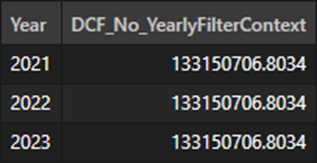
The output is straight forward; it produces a single metric indifferent of the year filter context (hence the name 😏). You can see an output below:

However, this leads us to the problem. Even though the output is a single metric, the measure generates a virtual in-memory table that spans multiple rows, requiring row context for financial-time-series evaluation. So how does one peer behind the curtain to ensure this table is evaluating compounding financial metrics correctly? In the next section, we will reveal a pattern to answer this exact question!
Option: Viewing Virtually Materialized Tables
The solution that I found useful is the following:
VALUATE
CALCULATETABLE(
	GENERATE(
		TABLE[COLUMNS] ...,
		ROW (
			"CALCULATIONS" , [Measures] , …
		)
	)
	, FILTERS …
)
Effectively, using CALCULATETABLE, materialize your table (row context) and measures in the first argument, and use the second argument to inject your filter context.
Transposing the example from above, the reformatted code looks like this:
EVALUATE
CALCULATETABLE(
	GENERATE(
		VAR __GrowthYears = SELECTEDVALUE( '_Growth Years'[Years] )
		RETURN
		GENERATESERIES(0,__GrowthYears-1,1),
		VAR __WACC = [Weighted Average Cost of Capital]
		VAR __GrowthRate = SELECTEDVALUE( '_Growth Rate'[Rate] )
		VAR __Last_FCFF = [FCFF - Last Available Year]
		VAR __TerminalValue = [Terminal Value]
		RETURN
			ROW (
				"FV" ,
					VAR __Index = [value]
	                VAR __FV = CALCULATE( __Last_FCFF * ( ( 1 + __GrowthRate ) ^ __Index ) )
	                RETURN __FV
				, "DCF" ,
					VAR __Index = [value]
	                VAR __FV = CALCULATE( __Last_FCFF * ( ( 1 + __GrowthRate ) ^ __Index ) )
	                VAR __PV = DIVIDE( __FV , ((1+__WACC) ^ __Index ) )
	                RETURN __PV
		    )
	)
	/*Growth*/
	, FILTER(KEEPFILTERS(VALUES('_Growth Rate'[Rate])), '_Growth Rate'[Rate] = .5)
	, FILTER(KEEPFILTERS(VALUES('_Growth Years'[Years])), '_Growth Years'[Years] = 7)
	, FILTER(KEEPFILTERS(VALUES('_Terminal Rate'[Rate])), '_Terminal Rate'[Rate] = .02 )
	/*WACC*/
	, FILTER(KEEPFILTERS(VALUES('_Equity Discount Rate'[Rate])), '_Equity Discount Rate'[Rate] = .10 )
	, FILTER(KEEPFILTERS(VALUES('_Debt Discount Rate'[Rate])), '_Debt Discount Rate'[Rate] = .10 )
	, FILTER(KEEPFILTERS(VALUES('_Equity Ratio'[Rate])), '_Equity Ratio'[Rate] = 1 )
	, FILTER(KEEPFILTERS(VALUES('_Tax Rate'[Rate])), '_Tax Rate'[Rate] = .26 )
)
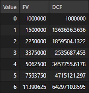
The output looks something like this:

One can see that for every year (column Value), a future value is being generated based on the growth rate and year and the present value is being discounted based on the WACC and year (again, reference the full article for more information on this equation). The final evaluation sums all these values (utilizing SUMX) and adds the terminal value; everything is working as intended!
The only disclosure I would give is to maintain where the variables go. For instance, the __GrowthYears variable needed to be before GENERATESERIES to ensure the table had access to the information, and the other variables (e.g., WACC) needed to be after GENERATESERIES to ensure the measures had access to this information. Play around with it and see what works for you!
Conclusion
In summary, this article provided another means for procuring virtual tables so users can ‘see behind the curtain’ – maintaining the row context and filter context for their DAX development.
About the Author:
William Rodriguez is the founder and principal consultant of Analytical Ants, an analytics company focused on procuring insights via data engineering, data science, and data analysis. William has led multi-million-dollar construction projects, acted as financial controller managing million-dollar monthly check productions, and built and deployed BI infrastructures at companies large ($30B Revenue) and ‘small’ ($60M Revenue). Academically, he has his master’s in business, two undergraduate business degrees, four active Microsoft certifications, and over 70 accredited SQLBI training hours. William loves spending time with his amazing family and knows that he would be nowhere without Christ.
Reach out to Analytical Ants LLC for all your data/analytical needs. We specialize in #DataEngineering #DataScience, and #DataAnalysis.

