Table of Contents:

• Accounting | Financial Overview
  • Intro
  • Basic Accounting Principles
• Financial Modeling with Business Intelligence
  • Star Schema
  • Basic Relationship Building
  • Advanced Modeling Techniques
• Conclusion
• Downloadable Content

Accounting | Financial Overview

Intro

Accounting and finance effectively are one in the same. As the old joke goes, ‘one holds the elephant’s trunk and another it’s tail; thinking they are touching different animals, they’re surprised when it’s revealed they are touching the same creature.’ Wait… that ‘joke’ may highlight exactly why people cannot see the forest from the trees.

Personally, I have completed YEARS of schooling in accounting and finance; yet seeing accounting and finance tie out completely never really ‘clicked’ until I had to functionally act as a controller ensuring that inputs rolled up to the outputs.

That’s my goal for you today. I want you to be able to take raw accounting data and transform that into financial reports that drive business forward. Ready? Let’s dive in!

Basic Accounting Principles

When preparing for this article, I found an old book of mine that covers basic accounting in a marvelous way. Therefore, I will be following a similar format to the book, “Accounting & Financial Management for Residential Construction, Fifth Edition” by Emma Shinn.

The basic financial accounting system is composed of the following key accounts: Assets, Liabilities, Owner’s Equity, Revenues, and Expenses. You can read more about those accounts here (Financial Accounting, Investopedia).

How these accounts relate with each other is through the accounting equation: Assets = Equities. Effectively, tangible assets equal intangible assets (i.e., investments and debt). Therefore, we get to the prime-time equation: Assets = Liabilities + Owner’s Equity. You can read more about the accounting equation here (Accounting Equation, Investopedia).

Assets increase with debits (Dr) and decrease with credits (Cr). The inverse is true for equities (L+OE). Equities increase with credits (Cr) and decrease with debits (Dr). You can read more about debits here (Debit, Investopedia) and credits here (Credit, Investopedia).

Finally, Owner’s equity can be split into two parts, Revenue and Expenses. Revenues increase with credits (Cr) and decrease with debits (Dr); Expenses increase with debits (Dr) and decrease with credits (Cr). This intuitively makes sense as you want more Revenues than Expenses, and a positive delta between the two will increase Owner’s Equity. There is an amazing image in the Accounting & Financial Management book (p.19) that gracefully summarizes the equation. It looks something like this:

Wow! Without knowing it, we successfully covered every ‘accounting type’ simply by reviewing the accounting equation. Assets, Liabilities, Owner’s Equity, Revenues, and Expenses – all accounted for (no pun intended)!

Now, these accounts materialize themselves categorically within bound parameters. For instance, within the ‘Assets’ category, you could have multiple asset types: cash, short-term investments, inventory, etc. Additionally, each subcategory could have multiple accounts. Example, your inventory could be subdivided into raw, work-in-progress, and finished goods. This hierarchical structure is called the Chart of Accounts (more information, Chart of Account, Investopedia). Recording individual transactions are done through journal entries (that maintain the accounting equation) and are logged to the General Ledger. More information can be found here (General Ledger and Double-Entry Accounting, Investopedia).

Lastly, summarizing the chart of accounts journal entries via the general ledger in different ways yields different financial metrics. Examples: the viability of a company, available cashflows, investments, and current liquidity positions. Three major reports that you will commonly see are Profit and Loss Statements, Balance Sheet Statements, and Cashflow Statements. These are the reports we will be covering in a subsequent article. You can find more about these financial statements via the following respective hyperlinks (Profit and Loss Statement, Cashflow Statement, Balance Sheet Statement, Investopedia)

WOW, talking about “eating an elephant one bite at a time”! If you understood that, AMAZING! You must have heard this before! If you’re completely lost, feel free to re-review and continue following along. Maybe you’re like me and things will ‘click’ with a tangible end-to-end example. That’s the beautiful thing about business intelligence, we need to understand the full system, and then we model reality with the data. It’s really that simple. Talking about modeling data, let’s dive into our next section where we will do just that, modeling the financial function.

Financial Modeling with Business Intelligence

Intro

By now, you’re a big shot financial guru 😏; or at least you have a fundamental understanding of how we get from point A to point B (namely, from journal entries to financial statements). The question remaining, how do we model this with data?

To tackle this problem, we will be introducing you to data engineering concepts of designing star schema models. We will be referencing the GOAT, Ralph Kimball, and his book, “The Data Warehouse Toolkit”. Before you balk, “I’m only an analyst!”; every analyst needs to be aware of how to structure their data properly for optimal performance. Now then, let’s begin.

Financial Modeling with Business Intelligence

Star Schema

The center of every BI implementation should be a star schema (Star Schema, Kimball). Namely, facts are surrounded by corresponding dimensions. What’s a fact? Great question. A fact table measures a business event at its lowest atomic granularity. An easy example is checking out at the grocery store. A transaction table for sales would have the date, time, receipt number, item number, and item quantity to describe a purchase. Ancillary information like the store location, manager salary, and promotions are all stored in separate dimensions that are connected to the fact table. Dimension tables describe the context for the transaction, which can be used to group, slice, and dice the transaction data. For example, you can use a dimension table to bind transactions based on promotion, or the brand of foods purchased. More information can be found here: Fact & Dimensions, Kimball and Star Schema Overview, Microsoft.

Let’s highlight the prior points with an example. The General Ledger is our fact table that describes the business function of accounting; individual journal entries are added to the General Ledger in batches. Each individual entry can have different accounts and other attributes. The quantity measurement of the fact table are the debits and credits columns. These are the columns we will use to aggregate for total amounts:

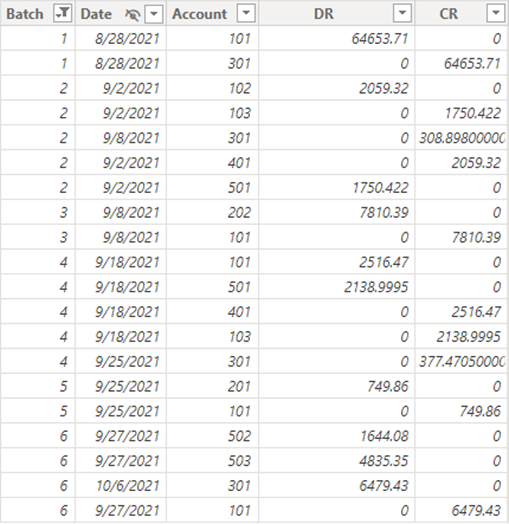
However, also note what is NOT here, there is a column for Account, yet no column for Account Description. Columns like these (i.e., additional attributes) are found on the dimension table, Chart of Account. This table is shown below:

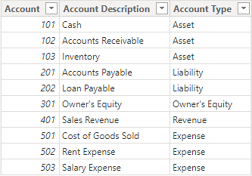
Following a Star Schema approach will optimize your model for performance and storage.

Basic Relationship Building

Relationship building is VITAL to data modeling. Ruining this could cause your model to no longer work. No pressure 😏. That’s why we are here to cover these concepts with you.

Typically, a fact table will have many attributes associated with a single record. While the individual record is unique to the table (i.e., the primary key), the attributes associated with that record might be replicated and shown on other records (i.e., foreign keys) (more information can be found here (Dimension Table Structure, Kimball). This relationship of having one record in the dimension table associated with many records in the fact table is called a one-to-many relationship.

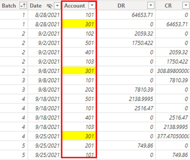
Let’s look at an example. In the fact table, there are multiple ‘301’ accounts listed in the column. This is because multiple transactions can be posted to the same account number. This is a foreign key in the fact table.

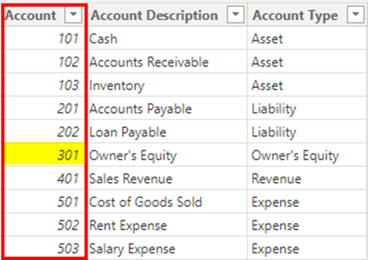
In the associated dimension table, there is only one ‘301’ account listed in the account column. This is because it’s a primary key for the dimension table (i.e., it perfectly describes that individual unit of the dimension – the account).

This can be represented in the ER diagram by the 1:* (Many) relationship as shown below.

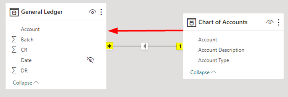
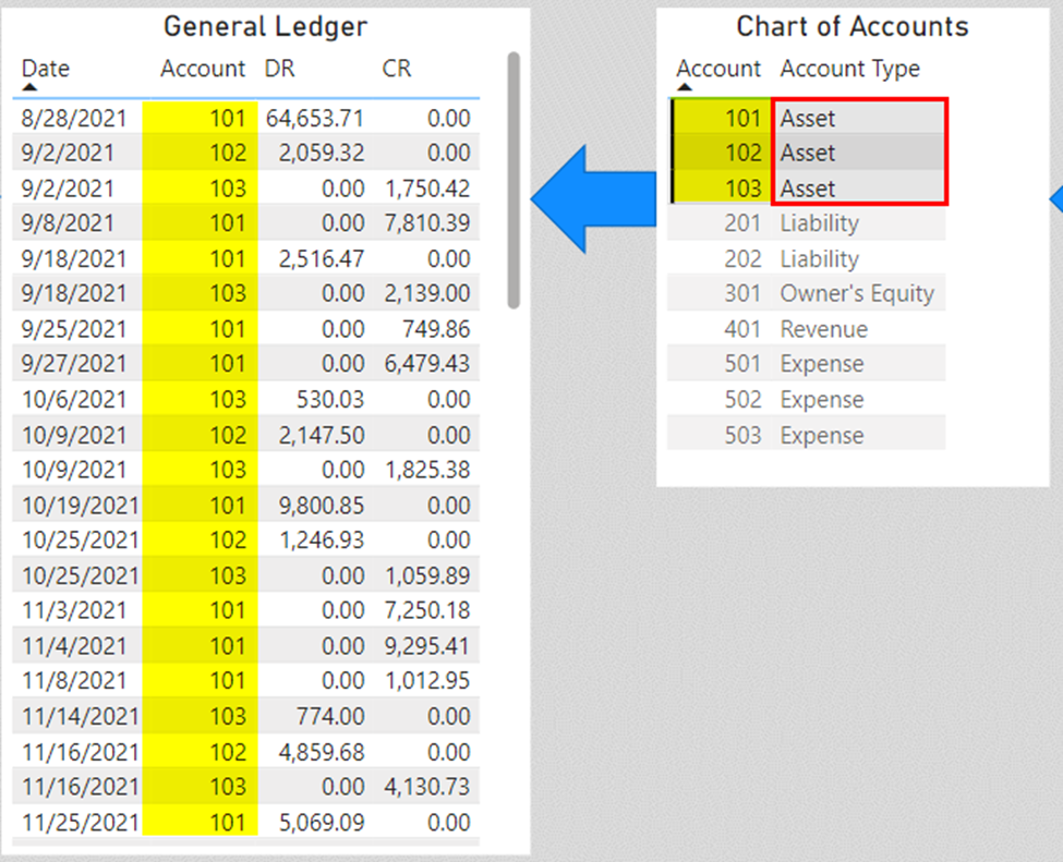
Please take note of the direction of the filter arrow, it goes from the 1 to the * (many) side. This means that selecting a dimension attribute will filter the fact table (not visa-versa). For example, if we select the ‘Asset’ value within the Chart of Accounts table (dimension), only ‘Asset’ accounts will show on the General Ledger table (fact).

Advanced Modeling Techniques

Below is our final model. Notice how the General Ledger is the centralized fact table with dimensions surrounding it; everything filters it. A keen eye will notice two abnormalities we haven’t covered. I’ll describe them below.

The two abnormalities are:

1. An Outrigger table: The Financial Statements table doesn’t connect to the fact table, but rather to a dimension table (i.e., Chart of Accounts). ‘Outriggering’ is a special normalizing/modeling technique that should only be used with intention. In this case, we need to establish a many-many relationships between the accounts in the fact table and the accounts in the Financial Statements table. The Chart of Accounts table is being utilized as our intermediary bridge table. More information on Outriggers, Snowflakes, and Bridges can be found here (Snowflakes, Outriggers, and Bridges, Kimball).
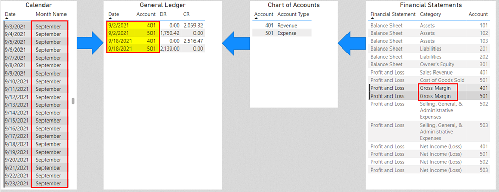
2. The bi-directional relationship between the Chart of Accounts and the Financial Statements table. Effectively, we need to be able to select a financial statement, or a row of a financial statement (e.g., Gross Margin on Profit and Loss Statement) and have that attribute filter down to the General Ledger table. For this, we need to utilize a bi-directional relationship so that the filter placed on the Financial Statements table can travel to the General Ledger table.

The best part about this model is that it functionally works as shown in the ER diagram when all tables are loaded to a report. For instance, if you select ‘September of 2021’ in the date dimension and ‘Gross Margin’ in the Financial Statements dimension, only September 2021 records for accounts 401 and 501 (i.e., Gross Margin) will return in the result set for the General Ledger. This is a nice introduction to row context and filter context- something we will need to talk about in our later articles (see more here: Row Context and Filter Context, SQLBI). For now, know that everything is working as intended!

Conclusion

We have covered the functional process of accounting and finance and have effectively translated this into a business intelligence model that we can use for reporting. Because we have effectively modeled the business process, this business intelligence model is transferable to any company or financial system. We will be deploying this model to both Excel and Power BI for financial reporting in subsequent posts. Be aware that implementations can vary slightly based on the tool (e.g., Excel vs. Power BI); however, the principles will hold constant.

We hope you enjoyed part one of this series, stay tuned for parts two and three!

Downloadable Content

————–

This article was created & published by William Rodriguez, Principal Architect at Analytical Ants

Reach out to Analytical Ants LLC for all your data/analytical needs. We specialize in #DataEngineering #DataScience, and #DataAnalysis. More Information can be found here.